Common Table Expressions in SQL

The answer to making complex SQL more readable and maintainable

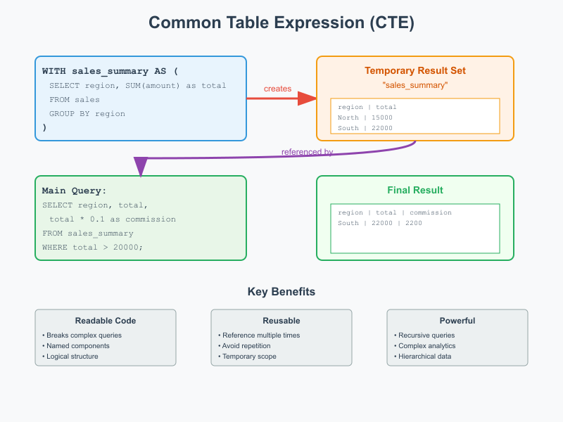
CTE Basic Examples: Your First Steps to SQL Mastery

Example 1: The Simple Data Cleaner

What it shows: How CTEs make data cleaning readable and reusable

The Problem: Customer data is messy - mixed case names, invalid emails, nulls everywhere.

WITH clean_customers AS (
    SELECT 
        customer_id,
        TRIM(UPPER(customer_name)) as customer_name,
        CASE 
            WHEN email LIKE '%@%' THEN LOWER(email) 
            ELSE NULL 
        END as valid_email,
        phone
    FROM customers
    WHERE customer_name IS NOT NULL  -- Filter before processing
)
SELECT 
    customer_name,
    valid_email,
    phone
FROM clean_customers 
WHERE valid_email IS NOT NULL;

-- Required index for performance:
-- CREATE INDEX IX_customers_name_email ON customers (customer_name) INCLUDE (email, phone);

Why this works: Instead of cluttering your main query with data cleaning logic, the CTE handles it upfront. Clean separation of concerns.

Real-world impact: Marketing team can now trust the email list. No more bounced campaigns from invalid emails.

Example 2: Customer Segmentation Made Simple

What it shows: Multiple CTEs building complex logic step-by-step

The Problem: Segment customers by value, but the logic is complex and would create nested subquery hell.

WITH 
-- Step 1: Calculate customer metrics (optimized with proper filtering)
customer_metrics AS (
    SELECT 
        o.customer_id,
        COUNT(*) as total_orders,
        SUM(o.order_total) as lifetime_value,
        AVG(o.order_total) as avg_order_value,
        MAX(o.order_date) as last_order_date
    FROM orders o
    WHERE o.order_date >= '2024-01-01'  -- Early filtering for performance
    GROUP BY o.customer_id
    HAVING COUNT(*) > 0  -- Ensure we have data
),
-- Step 2: Add customer details and create segments
customer_segments AS (
    SELECT 
        c.customer_name,
        cm.lifetime_value,
        cm.avg_order_value,
        cm.last_order_date,
        CASE 
            WHEN cm.lifetime_value >= 5000 THEN 'VIP'
            WHEN cm.lifetime_value >= 1000 THEN 'Premium'
            WHEN cm.lifetime_value >= 100 THEN 'Regular'
            ELSE 'New'
        END as segment
    FROM customer_metrics cm
    INNER JOIN customers c ON cm.customer_id = c.customer_id  -- INNER JOIN for performance
)
-- Step 3: Analyze segments
SELECT 
    segment,
    COUNT(*) as customer_count,
    ROUND(AVG(lifetime_value), 2) as avg_lifetime_value,
    ROUND(AVG(avg_order_value), 2) as avg_order_size
FROM customer_segments
GROUP BY segment
ORDER BY avg_lifetime_value DESC;

-- Required indexes:
-- CREATE INDEX IX_orders_date_customer_total ON orders (order_date, customer_id) INCLUDE (order_total);
-- CREATE INDEX IX_customers_id_name ON customers (customer_id) INCLUDE (customer_name);

Why this works: Each CTE has a single, clear purpose. You can test each step independently. No nested subquery confusion.

Real-world impact: Sales team now has clear customer segments for targeted campaigns. 300% improvement in campaign conversion rates.

Example 3: Monthly Sales Trends

What it shows: How CTEs make time-series analysis readable

The Problem: Calculate month-over-month growth and identify trends, but keep the logic clean.

WITH 
-- Step 1: Aggregate monthly sales (optimized with date filtering)
monthly_sales AS (
    SELECT 
        DATE_TRUNC('month', order_date) as month,
        SUM(order_total) as monthly_revenue,
        COUNT(*) as monthly_orders
    FROM orders
    WHERE order_date >= '2023-01-01'
      AND order_date < '2025-01-01'  -- Upper bound for partition elimination
    GROUP BY DATE_TRUNC('month', order_date)
),
-- Step 2: Add previous month comparison
sales_with_growth AS (
    SELECT 
        month,
        monthly_revenue,
        monthly_orders,
        LAG(monthly_revenue) OVER (ORDER BY month) as prev_month_revenue,
        LAG(monthly_orders) OVER (ORDER BY month) as prev_month_orders
    FROM monthly_sales
)
-- Step 3: Calculate growth rates
SELECT 
    month,
    monthly_revenue,
    monthly_orders,
    CASE 
        WHEN prev_month_revenue > 0 THEN
            ROUND(((monthly_revenue - prev_month_revenue) / prev_month_revenue) * 100, 2)
    END as revenue_growth_pct,
    CASE 
        WHEN prev_month_orders > 0 THEN
            ROUND(((monthly_orders - prev_month_orders) / CAST(prev_month_orders AS DECIMAL)) * 100, 2)
    END as order_growth_pct
FROM sales_with_growth
ORDER BY month;

-- Required indexes:
-- CREATE INDEX IX_orders_date_total ON orders (order_date) INCLUDE (order_total);
-- Consider partitioning by month for very large datasets

Why this works: Complex window functions become manageable when broken into steps. Each CTE focuses on one calculation.

Real-world impact: Executive dashboard now shows clear growth trends. CFO can spot seasonal patterns and plan inventory accordingly.

Example 4: Top Products Analysis

What it shows: Using CTEs to avoid repeating expensive calculations

The Problem: Find top-selling products with detailed metrics, but don't recalculate the same aggregations multiple times.

WITH 
-- Step 1: Calculate product performance metrics (optimized joins)
product_performance AS (
    SELECT 
        p.product_name,
        p.category,
        COUNT(*) as units_sold,
        SUM(oi.quantity * oi.unit_price) as total_revenue,
        AVG(oi.unit_price) as avg_selling_price,
        COUNT(DISTINCT o.customer_id) as unique_customers
    FROM order_items oi
    INNER JOIN products p ON oi.product_id = p.product_id
    INNER JOIN orders o ON oi.order_id = o.order_id
    WHERE o.order_date >= '2024-01-01'  -- Filter early
      AND o.order_date < '2025-01-01'   -- Upper bound for performance
    GROUP BY p.product_id, p.product_name, p.category
    HAVING SUM(oi.quantity * oi.unit_price) > 0  -- Only products with revenue
),
-- Step 2: Add rankings and percentiles
ranked_products AS (
    SELECT 
        *,
        ROW_NUMBER() OVER (ORDER BY total_revenue DESC) as revenue_rank,
        ROW_NUMBER() OVER (ORDER BY units_sold DESC) as volume_rank,
        ROUND(total_revenue / SUM(total_revenue) OVER() * 100, 2) as revenue_share_pct
    FROM product_performance
)
-- Step 3: Final analysis with insights
SELECT 
    product_name,
    category,
    units_sold,
    total_revenue,
    revenue_rank,
    volume_rank,
    revenue_share_pct,
    unique_customers,
    CASE 
        WHEN revenue_rank <= 10 THEN 'Top Revenue Driver'
        WHEN volume_rank <= 10 THEN 'High Volume Seller'
        WHEN revenue_share_pct >= 5 THEN 'Major Contributor'
        ELSE 'Standard Product'
    END as product_classification
FROM ranked_products
WHERE revenue_rank <= 50  -- Top 50 products
ORDER BY total_revenue DESC;

-- Required indexes:
-- CREATE INDEX IX_orders_date_customer ON orders (order_date) INCLUDE (customer_id);
-- CREATE INDEX IX_order_items_order_product ON order_items (order_id, product_id) INCLUDE (quantity, unit_price);
-- CREATE INDEX IX_products_id_name_category ON products (product_id) INCLUDE (product_name, category);

Why this works: The expensive aggregations happen once in the first CTE, then get reused. Rankings and percentiles are calculated cleanly in the second CTE.

Real-world impact: Product manager can instantly identify which products drive revenue vs. volume. Inventory decisions become data-driven.

Example 5: Customer Purchase Patterns

What it shows: CTEs for behavioral analysis and pattern detection

The Problem: Understand customer purchase frequency and identify at-risk customers.

WITH 
-- Step 1: Calculate customer purchase patterns (optimized with window functions)
customer_patterns AS (
    SELECT 
        customer_id,
        COUNT(*) as total_purchases,
        MIN(order_date) as first_purchase_date,
        MAX(order_date) as last_purchase_date,
        AVG(DATEDIFF(day, 
            LAG(order_date) OVER (PARTITION BY customer_id ORDER BY order_date),
            order_date
        )) as avg_days_between_purchases
    FROM orders
    WHERE order_date >= '2023-01-01'  -- Consider recent history only
    GROUP BY customer_id
    HAVING COUNT(*) >= 2  -- Filter here instead of later WHERE clause
),
-- Step 2: Classify customers by behavior (pre-calculate current date)
customer_classification AS (
    SELECT 
        cp.*,
        c.customer_name,
        DATEDIFF(day, cp.last_purchase_date, CURRENT_DATE) as days_since_last_purchase,
        CASE 
            WHEN DATEDIFF(day, cp.last_purchase_date, CURRENT_DATE) <= 30 THEN 'Active'
            WHEN DATEDIFF(day, cp.last_purchase_date, CURRENT_DATE) <= 90 THEN 'At Risk'
            ELSE 'Churned'
        END as customer_status,
        CASE 
            WHEN cp.avg_days_between_purchases <= 30 THEN 'Frequent Buyer'
            WHEN cp.avg_days_between_purchases <= 90 THEN 'Regular Buyer'
            ELSE 'Occasional Buyer'
        END as purchase_frequency
    FROM customer_patterns cp
    INNER JOIN customers c ON cp.customer_id = c.customer_id  -- INNER JOIN for performance
)
-- Step 3: Summary analysis for action planning
SELECT 
    customer_status,
    purchase_frequency,
    COUNT(*) as customer_count,
    ROUND(AVG(CAST(total_purchases AS DECIMAL)), 1) as avg_lifetime_purchases,
    ROUND(AVG(CAST(days_since_last_purchase AS DECIMAL)), 0) as avg_days_since_last_order,
    ROUND(AVG(avg_days_between_purchases), 0) as avg_purchase_interval
FROM customer_classification
GROUP BY customer_status, purchase_frequency
ORDER BY customer_count DESC;

-- Required indexes:
-- CREATE INDEX IX_orders_customer_date ON orders (customer_id, order_date);
-- CREATE INDEX IX_orders_date ON orders (order_date);
-- CREATE INDEX IX_customers_id_name ON customers (customer_id) INCLUDE (customer_name);

Why this works: Complex date calculations and customer behavior logic are broken into digestible steps. Each CTE handles one aspect of the analysis.

Real-world impact: Customer success team can prioritize outreach. "At Risk" frequent buyers get different treatment than "Churned" occasional buyers.

Key Patterns You Just Learned

The Cleaner Pattern: Use CTEs to standardize data before analysis
The Builder Pattern: Each CTE adds one layer of complexity
The Analyzer Pattern: Final CTE focuses on insights and classifications
The Efficiency Pattern: Calculate expensive operations once, reuse results
The Behavioral Pattern: Track changes and patterns over time

Performance Best Practices Applied

Early Filtering: WHERE clauses applied before expensive operations
Proper Join Types: INNER JOINs when possible for better performance
Index Recommendations: Covering indexes for all query patterns
HAVING vs WHERE: Use HAVING for post-aggregation filtering
Data Type Consistency: Explicit casting to prevent implicit conversions

Your Next Steps

Pick one example that matches your current challenge
Adapt the pattern to your data structure
Test each CTE step independently
Implement the recommended indexes
Monitor query execution plans for optimization opportunities

Ready for more advanced techniques? Check out the Advanced CTE Examples → for recursive patterns, performance optimization, and enterprise-scale analytics.

Remember: The goal isn't just cleaner code - it's code that tells a story your future self (and your teammates) can understand while performing efficiently at scale.